Review: Generic Parallel Functional Programming
Today we’re heading back into the Elliottverse — a beautiful world where programming is principled and makes sense. The paper of the week is Conal Elliott’s Generic Parallel Functional Programming, which productively addresses the duality between “easy to reason about” and “fast to run.”
Consider the case of a right-associated list, we can give a scan of it in linear time and constant space:
module ExR where
  data RList (A : Set) : Set where
    RNil : RList A
    _◁_ : A → RList A → RList A

  infixr 5 _◁_

  scanR : ⦃ Monoid A ⦄ → RList A → RList A
  scanR = go mempty
    where
      go : ⦃ Monoid A ⦄ → A → RList A → RList A
      go acc RNil = RNil
      go acc (x ◁ xs) = acc ◁ go (acc <> x) xs
This is a nice functional algorithm that runs in \(O(n)\) time, and requires \(O(1)\) space. However, consider the equivalent algorithm over left-associative lists:
module ExL where
  data LList (A : Set) : Set where
    LNil : LList A
    _▷_ : LList A → A → LList A

  infixl 5 _▷_

  scanL : ⦃ Monoid A ⦄ → LList A → LList A
  scanL = proj₁ ∘ go
    where
      go : ⦃ Monoid A ⦄ → LList A → LList A × A
      go LNil = LNil , mempty
      go (xs ▷ x) =
        let xs' , acc = go xs
         in xs' ▷ acc , x <> acc
While scanL is also \(O(n)\) in its runtime, it is not amenable to tail call optimization, and thus also requires \(O(n)\) space. Egads!
You are probably not amazed to learn that different ways of structuring data lead to different runtime and space complexities. But it’s a more interesting puzzle than it sounds; because RList and LList are isomorphic! So what gives?
Reed’s pithy description here is
Computation time doesn’t respect isos
Exploring that question with him has been very illuminating. Math is deeply about extentionality; two mathematical objects are equivalent if their abstract interfaces are indistinguishable. Computation… doesn’t have this property. When computing, we care a great deal about runtime performance, which depends on fiddly implementation details, even if those aren’t externally observable.
In fact, as he goes on to state, this is the whole idea of denotational design. Figure out the extensional behavior first, and then figure out how to implement it.
This all harkens back to my review of another of Elliott’s papers, Adders and Arrows, which starts from the extensional behavior of natural addition (encoded as the Peano naturals), and then derives a chain of proofs showing that our everyday binary adders preserve this behavior.
Anyway, let’s switch topics and consider a weird fact of the world. Why do so many parallel algorithms require gnarly array indexing? Here’s an example I found by googling for “parallel c algorithms cuda”:
__global__ void stencil_1d(int *in, int *out) {
  __shared__ int temp[BLOCK_SIZE + 2 * RADIUS];
  int gindex = threadIdx.x + blockIdx.x * blockDim.x;
  int lindex = threadIdx.x + RADIUS;
  temp[lindex] = in[gindex];
  if (threadIdx.x < RADIUS) {
    temp[lindex - RADIUS] = in[gindex - RADIUS];
    temp[lindex + BLOCK_SIZE] =
    in[gindex + BLOCK_SIZE];
  }
  __syncthreads();
  int result = 0;
  for (int offset = -RADIUS ; offset <= RADIUS ; offset++)
    result += temp[lindex + offset];
  out[gindex] = result;
}
and here’s another, expressed as an “easy induction” recurrence relation, from Richard E Ladner and Michael J Fischer. Parallel prefix computation:
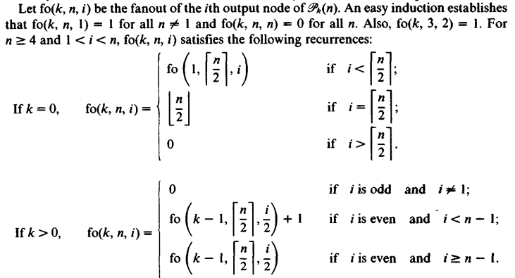
Sweet lord. No wonder we’re all stuck pretending our computer machines are single threaded behemoths from the 1960s. Taking full advantage of parallelism on modern CPUs must require a research team and five years!
But it’s worth taking a moment and thinking about what all of this janky indexing must be doing. Whatever algorithm is telling the programmer which indices to write where necessarily must be providing a view on the data. That is, the programmer has some sort of “shape” in mind for how the problem should be subdivided, and the indexing is an implementation of accessing the raw array elements in the desired shape.
At risk of beating you on the head with it, this array indexing is a bad implementation of a type system. Bad because it’s something the implementer needed to invent by hand, and is not in any form that the compiler can help ensure the correctness of.
That returns us to the big contribution of Generic Function Parallel Algorithms, which is a technique for decoupling the main thrust of an algorithm from extentionally-inconsequential encodings of things. The idea is to implement the algorithm on lots of trivial data structures, and then compose those small pieces together to get a class of algorithms.
Generic Representations
The first step is to determine which trivial data structures we need to support. Following the steps of Haskell’s GHC.Generics module, we can decompose any Haskell98 data type as compositions of the following pieces:
data Rep : Set₁ where
  V : Rep
  U : Rep
  K : Set → Rep
  Par : Rep
  Rec : (Set → Set) → Rep
  _:+:_ : Rep → Rep → Rep
  _:*:_ : Rep → Rep → Rep
  _:∘:_ : Rep → Rep → Rep
which we can embed in Set via Represent:
open import Data.Empty
open import Data.Sum
open import Data.Unit hiding (_≤_)

record Compose (F G : Set → Set) (A : Set) : Set where
  constructor compose
  field
    composed : F (G A)
open Compose

Represent : Rep → Set → Set
Represent V a         = ⊥
Represent U a         = ⊤
Represent (K x) a     = x
Represent Par a       = a
Represent (Rec f) a   = f a
Represent (x :+: y) a = Represent x a ⊎ Represent y a
Represent (x :*: y) a = Represent x a × Represent y a
Represent (x :∘: y) a = Compose (Represent x) (Represent y) a
If you’ve ever worked with GHC.Generics, none of this should be very exciting. We can bundle everything together, plus an iso to transform to and from the Represented type:
record Generic (F : Set → Set) : Set₁ where
  field
    RepOf : Rep
    from  : F A → Represent RepOf A
    to    : Represent RepOf A → F A
open Generic ⦃ ... ⦄

GenericRep : (F : Set → Set) → ⦃ Generic F ⦄ → Set → Set
GenericRep _ = Represent RepOf
Agda doesn’t have any out-of-the-box notion of -XDeriveGeneric, which seems like a headache at first blush. It means we need to explicitly write out a RepOf and from/to pairs by hand, like peasants. Surprisingly however, needing to implement by hand is beneficial, as it reminds us that RepOf is not uniquely determined!
A good metaphor here is the number 16, which stands for some type we’d like to generify. A RepOf for 16 is an equivalent representation for 16. Here are a few:
- \(2+(2+(2+(2+(2+(2+(2+2))))))\)
- \(((2+2)*2)+(((2+2)+2)+2)\)
- \(2 \times 8\)
- \(8 \times 2\)
- \((4 \times 2) \times 2\)
- \((2 \times 4) \times 2\)
- \(4 \times 4\)
- \(2^4\)
- \(2^{2^2}\)
And there are lots more! Each of \(+\), \(\times\) and exponentiation corresponds to a different way of building a type, so every one of these expressions is a distinct (if isomorphic) type with 16 values. Every single possible factoring of 16 corresponds to a different way of dividing-and-conquering, which is to say, a different (but related) algorithm.
The trick is to define our algorithm inductively over each Set that can result from Represent. We can then pick different algorithms from the class by changing the specific way of factoring our type.
Left Scans
Let’s consider the case of left scans. I happen to know it’s going to require Functor capabilities, so we’ll also define that:
record Functor (F : Set 𝓁 → Set 𝓁) : Set (lsuc 𝓁) where
  field
    fmap : {A B : Set 𝓁} → (A → B) → F A → F B

record LScan (F : Set → Set) : Set₁ where
  field
    overlap ⦃ func ⦄ : Functor F
    lscan : ⦃ Monoid A ⦄ → F A → F A × A

open Functor ⦃  ...  ⦄
open LScan ⦃ ... ⦄
What’s with the type of lscan? This thing is an exclusive scan, so the first element is always mempty, and thus the last elemenet is always returned as proj₂ of lscan.
We need to implement LScan for each Representation, and because there is no global coherence requirement in Agda, we can define our Functor instances at the same time.
The simplest case is void which we can scan because we have a ⊥ in negative position:
instance
  lV : LScan (\a → ⊥)
  lV .func .fmap f x = ⊥-elim x
  lV .lscan ()
⊤ is also trivial. Notice that there isn’t any a inside of it, so our final accumulated value must be mempty:
  lU : LScan (\a → ⊤)
  lU .func .fmap f x = x
  lU .lscan x = x , mempty
The identity functor is also trivial. Except this time, we do have a result, so it becomes the accumulated value, and we replace it with how much we’ve scaned thus far (nothing):
  lP : LScan (\a → a)
  lP .func .fmap f = f
  lP .lscan x = mempty , x
Coproducts are uninteresting; we merely lift the tag:
  l+ : ⦃ LScan F ⦄ → ⦃ LScan G ⦄ → LScan (\a → F a ⊎ G a)
  l+ .func .fmap f (inj₁ y) = inj₁ (fmap f y)
  l+ .func .fmap f (inj₂ y) = inj₂ (fmap f y)
  l+ .lscan (inj₁ x) =
    let x' , y = lscan x
     in inj₁ x' , y
  l+ .lscan (inj₂ x) =
    let x' , y = lscan x
     in inj₂ x' , y
And then we come to the interesting cases. To scan the product of F and G, we notice that every left scan of F is a prefix of F × G (because F is on the left.) Thus, we can use lscan F directly in the result, and need only adjust the results of lscan G with the accumulated value from F:
  l* : ⦃ LScan F ⦄ → ⦃ LScan G ⦄ → LScan (\a → F a × G a)
  l* .func .fmap f x .proj₁ = fmap f (x .proj₁)
  l* .func .fmap f x .proj₂ = fmap f (x .proj₂)
  l* .lscan (f-in , g-in) =
    let f-out , f-acc = lscan f-in
        g-out , g-acc = lscan g-in
     in (f-out , fmap (f-acc <>_) g-out) , f-acc <> g-acc
l* is what makes the whole algorithm parallel. It says we can scan F and G in parallel, and need only a single join node at the end to stick f-acc <>_ on at the end. This parallelism is visible in the let expression, where there is no data dependency between the two bindings.
Our final generic instance of LScan is over composition. Howevef, we can’t implement LScan for every composition of functors, since we require the ability to “zip” two functors together. The paper is pretty cagey about exactly what Zip is, but after some sleuthing, I think it’s this:
record Zip (F : Set → Set) : Set₁ where
  field
    overlap ⦃ func ⦄ : Functor F
    zip : {A B : Set} → F A → F B → F (A × B)
open Zip ⦃ ... ⦄
That looks a lot like being an applicative, but it’s missing pure and has some weird idempotent laws that are not particularly relevant today. We can define some helper functions as well:
zipWith : ∀ {A B C} → ⦃ Zip F ⦄ → (A → B → C) → F A → F B → F C
zipWith f fa fb = fmap (uncurry f) (zip fa fb)

unzip : ⦃ Functor F ⦄ → {A B : Set} → F (A × B) → F A × F B
unzip x = fmap proj₁ x , fmap proj₂ x
Armed with all of this, we can give an implementation of lscan over functor composition. The idea is to lscan each inner functor, which gives us an G (F A × A). We can then unzip that, whose second projection is then the totals of each inner scan. If we scan these totals, we’ll get a running scan for the whole thing; and all that’s left is to adjust each.
instance
  l∘ : ⦃ LScan F ⦄ → ⦃ LScan G ⦄ → ⦃ Zip G ⦄ → LScan (Compose G F)
  l∘ .func .fmap f = fmap f
  l∘ .lscan (compose gfa) =
    let gfa' , tots = unzip (fmap lscan gfa)
        tots' , tot = lscan tots
        adjustl t = fmap (t <>_)
    in compose (zipWith adjustl tots' gfa') , tot
And we’re done! We now have an algorithm defined piece-wise over the fundamental ADT building blocks. Let’s put it to use.
Dividing and Conquering
Let’s pretend that Vecs are random access arrays. We’d like to be able to build array algorithms out of our algorithmic building blocks. To that end, we can make a typeclass corresponding to types that are isomorphic to arrays:
open import Data.Nat
open import Data.Vec hiding (zip; unzip; zipWith)

record ArrayIso (F : Set → Set) : Set₁ where
  field
    Size : ℕ
    deserialize : Vec A Size → F A
    serialize : F A → Vec A Size
    -- also prove it's an iso

open ArrayIso ⦃ ... ⦄
There are instances of ArrayIso for the functor building blocks (though none for :+: since arrays are big records.) We can now use an ArrayIso and an LScan to get our desired parallel array algorithms:
genericScan
    : ⦃ Monoid A ⦄
    → (rep : Rep)
    → ⦃ d : ArrayIso (Represent rep) ⦄
    → ⦃ LScan (Represent rep) ⦄
    → Vec A (Size ⦃ d ⦄)
    → Vec A (Size ⦃ d ⦄) × A
genericScan _ ⦃ d = d ⦄ x =
  let res , a = lscan (deserialize x)
   in serialize ⦃ d ⦄ res , a
I think this is the first truly dependent type I’ve ever written. We take a Rep corresponding to how we’d like to divvy up the problem, and then see if the Represent of that has ArrayIso and LScan instances, and then give back an algorithm that scans over arrays of the correct Size.
Finally we’re ready to try this out. We can give the RList implementation from earlier:
▷_ : Rep → Rep
▷_ a = Par :*: a

_ : ⦃ Monoid A ⦄ → Vec A 4 → Vec A 4 × A
_ = genericScan (▷ ▷ ▷ Par)
or the LList instance:
_◁ : Rep → Rep
_◁ a = a :*: Par

_ : ⦃ Monoid A ⦄ → Vec A 4 → Vec A 4 × A
_ = genericScan (Par ◁ ◁ ◁)
But we can also come up with more interesting strategies as well. For example, we can divvy up the problem by left-associating the first half, and right-associating the second:
_ : ⦃ Monoid A ⦄ → Vec A 8 → Vec A 8 × A
_ = genericScan ((Par ◁ ◁ ◁) :*: (▷ ▷ ▷ Par))
This one probably isn’t an efficient algorithm, but it’s cool that we can express such a thing so succinctly. Probably of more interest is a balanced tree over our array:
_ : ⦃ Monoid A ⦄ → Vec A 16 → Vec A 16 × A
_ = let ⌊_⌋ a = a :*: a
     in genericScan (⌊ ⌊ ⌊ ⌊ Par ⌋ ⌋ ⌋ ⌋)
The balanced tree over products is interesting, but what if we make a balanced tree over composition? In essence, we can split the problem into chunks of \(2^(2^n)\) amounts of work via Bush:
{-# NO_POSITIVITY_CHECK #-}
data Bush : ℕ → Set → Set where
  twig : A × A → Bush 0 A
  bush : {n : ℕ} → Bush n (Bush n A) → Bush (suc n) A
Which we won’t use directly, but can use it’s Rep:
_ : ⦃ Monoid A ⦄ → Vec A 16 → Vec A 16 × A
_ = let pair = Par :*: Par
     in genericScan ((pair :∘: pair) :∘: (pair :∘: pair))
The paper compares several of these strategies for dividing-and-conquering. In particular, it shows that we can minimize total work via a left-associated ⌊_⌋ strategy, but maximize parallelism with a right-associated ⌊_⌋. And using the Bush from earlier, we can get a nice middle ground.
Very Quick FFTs
The paper follows up, applying this approach to implementations of the fast fourier transform. There, the Bush approach gives constant factor improvments for both work and parallelism, compared to all previously known algorithms.
Results like these are strong evidence that Elliott is actually onto something with his seemingly crazy ideas that computation should be elegant and well principled. Giving significant constant factor improvements to well-known, extremely important algorithms mostly for free is a true superpower, and is worth taking extremely seriously.
Fighting Against Publication Bias
Andrew McKnight and I tried to use this same approach to get a nice algorithm for sorting, hoping that we could get well-known sorting algorithms to fall out as special cases of our more general functor building blocks. We completely failed on this front, namely because we couldn’t figure out how to give an instance for product types. Rather alarmingly, we’re not entirely sure why the approach failed there; maybe it was just not thinking hard enough.
Another plausible idea is that sorting requires branching, and that this approach only works for statically-known codepaths.
Future Work
Andrew and I spent a good chunk of the week thinking about this problem, and we figure there are solid odds that you could automatically discover these generic algorithmic building blocks from a well-known algorithm. Here’s the sketch:
Use the well-known algorithm as a specification, instantiate all parameters at small types and see if you can find instances of the algorithm for the functor building blocks that agree with the spec. It seems like you should be able to use factorization of the input to target which instances you’re looking for.
Of course, once you have the algorithmic building blocks, conventional search techniques can be used to optimize any particular goal you might have.